Capacitated Facility Location Problem(CFLP)问题是一个典型的NP-Hard问题,该问题的描述如下,
- 给定
N个设施(facility)和M位顾客(customer),每个设施有一个最大容量s,并且可以选择开启或关闭,开启有一个开启费用f。 - 每位顾客有一个需求
d,需要被某个或某些个设施满足,某个设施满足的需求数不得超过其最大容量s。 - 每个设施到每个顾客都有一个满足费用
c,即满足某个顾客单位需求的费用。 - 最小化满足所有顾客所有需求的总费用。
分析
引入如下的数学符号,
- $N$表示设施数,$M$表示顾客数。
- $s_i, \forall i = 0,…,N-1$表示设施$i$的最大容量。
- $f_i, \forall i = 0,…,N-1$表示设施$i$的开启费用。
- $d_i, \forall i = 0,…,M-1$表示顾客$i$的需求。
- $c_{ij}, \forall i = 0,…,N-1, j = 0,…,M-1$表示设施$i$满足顾客$j$单位需求所需费用。
- 注:一般而言,用$c_{ij}$表示的是满足顾客所有需求所需费用,这里为避免引入除法和分数采用单位需求。
并将CFLP的解表示为,
- $x_i, \forall i = 0,…,N-1, x_i \in \{0,1\}$表示设施$i$的开启状况,1表示开启,0表示关闭。
- $y_{ij}, \forall i = 0,…,N-1, j=0,…,M-1$表示设施$i$满足顾客$j$的需求数。
那么CFLP可以表示为如下的最优化问题,
$$
min \sum_{i=0}^{N-1}\sum_{j=0}^{M-1}c_{ij}y_{ij} + \sum_{i=0}^{N-1}f_ix_i \quad s.t. \\
\begin{align}
y_{ij} \ge 0 & \quad \forall i=0,…,N-1, j=0,…,M-1 \\
\sum_{j=0}^{M-1}y_{ij} \le s_ix_i & \quad \forall i=0,…,N-1 \\
\sum_{i=0}^{N-1}y_{ij} = d_j & \quad \forall j=0,…,M-1 \\
x_i \in \{0,1\} & \quad \forall i=0,…,N-1
\end{align}
$$
CFLP的条件比较多,但您可以将解过程分为两个部分,
- 开启一些设施(求解$x$)。
- 决定每个顾客在每个设施中满足需求的数量(将用户需求赋值给设施,求解$y$)。
其中,开启设施共有$2^N$种可能性,也是使得这个问题无法在多项式时间内求解的关键因素。当开启的设施已经被选定时,可以采用如下的贪心策略对设施赋值,
- 在已开启且还有容量剩余的设施和还未被满足需求的顾客中选择费用最低的设施-顾客对,尽可能地满足该顾客,直到所有顾客都被满足。
- 若该顾客已满足,则将顾客移出考虑范围;若该顾客未被满足,则设施已达到最大容量,将该设施移出考虑范围;特别的,恰好满足时,同时移除设施和顾客;此时如果还有顾客未被满足,则返回1,否则结束过程。
因此,考虑的重点在于选择哪些设施进行开启,下面将着重阐述若干个策略。
实现
- 实现框架:Golang+Cobra命令行程序
问题的表示
问题包含$N,M,s,f,d,c$五个变量,其中$N,M$用两个整数表示,$s,f$分别用一个长度为$N$的一维数组表示,$d$用一个长度为$M$的一维数组表示,$c$采用一个$N \times M$的二维数组表示,结构如下,
1 | // Problem contains data of a CFLP. |
注:为了计算方便,在读取数据的时候计算了总需求并储存在变量TotalDemand中。
易得,读取数据的时间复杂度为$O(NM)$,空间复杂度为$O(NM)$。
解的表示
一个解包含设施的开启信息$x$和用户需求的赋值信息$y$,分别使用一个长度为$N$的一维数组和一个$N \times M$的二维数组表示,结构如下,
1 | // Solution represents a solution of a CFLP. |
注:添加了RunTime记录运行时间。
当X确定时,采用上面提到的贪心策略进行需求赋值的代码过程如下,
1 | // Assign assigns demands to facility based on current opened facilities. |
可见,该过程须要临时保留每个设施被占用的容量以及每个顾客剩余的需求,因此空间复杂度为$O(N+M)$。
时间上,每次循环内需要便利所有符合条件的设施-用户对的费用,循环内时间复杂度为$O(NM)$,而每次循环过后必定有一个用户得到满足或者某个设施占用容量达到最大,所以循环次数不会超过设施数和用户数的总和,因此整个过程的时间复杂度为$O(NM(N+M))$。
Greedy 贪心策略
在选择设施上进行贪心策略显然不是最优的,但贪心策略的优点在于运行速度快,能够很快地得到一个参考结果,用于对比其他算法的解。
贪心策略非常简单,
- 选择设施中未开启的开启费用最少的设施,开启它。
- 若开启的设施的总容量小于顾客的总需求,回到1,否则结束。
运行代码片段如下,
1 | func (s *Solver) solveByGreedy() *Solution { |
复杂度分析
整个算法的流程如下,
- 初始化解($O(MN)$)。
- 寻找未开启设施中开启费用最低的设施($O(N)$)。
- 若开启的设施无法满足所用顾客的需要,返回2。(最多返回$N$次)
- 需求赋值($O(MN(M+N))$)。
因此,贪心策略的时间复杂度为$O(N^2 + MN(M+N))$。
由于整个过程仅需要保持一个解,空间复杂度为$O(MN)$。
实验结果
在71个问题的问题集上的实验结果如下,
| Result | Time(s) | |
|---|---|---|
| p1 | 12989.953 | 0.00004 |
| p2 | 9288.850 | 0.00007 |
| p3 | 10488.850 | 0.00008 |
| p4 | 11688.850 | 0.00036 |
| p5 | 10902.060 | 0.00008 |
| p6 | 9832.666 | 0.00007 |
| p7 | 11432.666 | 0.00006 |
| p8 | 13032.666 | 0.00016 |
| p9 | 10980.250 | 0.00010 |
| p10 | 10458.043 | 0.00009 |
| p11 | 11458.043 | 0.00006 |
| p12 | 12458.043 | 0.00004 |
| p13 | 11015.048 | 0.00028 |
| p14 | 8514.791 | 0.00006 |
| p15 | 10114.791 | 0.00012 |
| p16 | 11714.791 | 0.00009 |
| p17 | 10295.318 | 0.00006 |
| p18 | 8543.171 | 0.00007 |
| p19 | 10143.171 | 0.00013 |
| p20 | 11743.171 | 0.00009 |
| p21 | 12235.528 | 0.00022 |
| p22 | 11363.414 | 0.00009 |
| p23 | 12563.414 | 0.00005 |
| p24 | 13763.414 | 0.00008 |
| p25 | 78338.667 | 0.00039 |
| p26 | 63710.947 | 0.00032 |
| p27 | 65310.947 | 0.00032 |
| p28 | 66910.947 | 0.00034 |
| p29 | 65258.221 | 0.00040 |
| p30 | 54927.860 | 0.00038 |
| p31 | 56927.860 | 0.00043 |
| p32 | 58927.860 | 0.00145 |
| p33 | 77701.857 | 0.00035 |
| p34 | 53887.154 | 0.00033 |
| p35 | 55487.154 | 0.00035 |
| p36 | 57087.154 | 0.00065 |
| p37 | 101999.196 | 0.00024 |
| p38 | 73636.480 | 0.00020 |
| p39 | 74636.480 | 0.00022 |
| p40 | 75636.480 | 0.00020 |
| p41 | 7276.556 | 0.00021 |
| p42 | 8068.351 | 0.00010 |
| p43 | 6383.929 | 0.00009 |
| p44 | 7995.223 | 0.00021 |
| p45 | 8089.250 | 0.00013 |
| p46 | 6915.251 | 0.00009 |
| p47 | 7705.325 | 0.00015 |
| p48 | 7874.275 | 0.00019 |
| p49 | 6960.522 | 0.00009 |
| p50 | 12441.358 | 0.00025 |
| p51 | 9382.546 | 0.00034 |
| p52 | 13378.456 | 0.00016 |
| p53 | 12650.089 | 0.00019 |
| p54 | 10536.867 | 0.00016 |
| p55 | 12258.408 | 0.00019 |
| p56 | 32522.303 | 0.00113 |
| p57 | 37322.303 | 0.00119 |
| p58 | 48522.303 | 0.00209 |
| p59 | 30606.927 | 0.00110 |
| p60 | 37243.427 | 0.00082 |
| p61 | 40543.427 | 0.00142 |
| p62 | 48243.427 | 0.00082 |
| p63 | 31843.780 | 0.00091 |
| p64 | 34081.806 | 0.00061 |
| p65 | 36481.806 | 0.00061 |
| p66 | 42081.806 | 0.00063 |
| p67 | 32210.447 | 0.00096 |
| p68 | 38955.963 | 0.00073 |
| p69 | 41955.963 | 0.00071 |
| p70 | 48955.963 | 0.00128 |
| p71 | 31843.976 | 0.00096 |
Brute Force 暴力求解
在$N$比较小时,可以使用暴力求解的方式,即枚举所有设施开启和关闭的可能性(共$2^N$种可能)。暴力求解的时间复杂度为$O(2^N)$,因此当$N$比较大时,这种方法是不适用的,但是暴力求解可以在不清楚最优解的情况下找到一个理论上的最优解,用于比较分析其他求解算法。
暴力求解的代码过程如下,
1 | func (s *Solver) solveByBruteForce() *Solution { |
过程中,通过一个整数$c, 0 \le c < 2^N$来表示$N$个设施的唯一一种开关状态,以其二进制数中的1表示开启,0表示关闭,因此遍历c即可遍历所有情况。
时间复杂度:$O(2^N)$
空间复杂度:$O(MN)$
实际实验过程中,当$N > 20$时运行时间已经不可接受,应当使用其它的一些算法。
实验结果
| Result | Time(s) | |
|---|---|---|
| p1 | 8899.287 | 0.01975 |
| p2 | 7943.402 | 0.01708 |
| p3 | 9543.402 | 0.01890 |
| p4 | 10947.538 | 0.01488 |
| p5 | 8928.489 | 0.00602 |
| p6 | 7729.489 | 0.00627 |
| p7 | 9529.489 | 0.00606 |
| p8 | 11259.081 | 0.00579 |
| p9 | 8460.030 | 0.03576 |
| p10 | 7617.000 | 0.03523 |
| p11 | 9103.286 | 0.03549 |
| p12 | 10363.911 | 0.03088 |
| p13 | 8245.910 | 63.38475 |
| p14 | 7125.641 | 63.63613 |
| p15 | 8856.372 | 62.66329 |
| p16 | 10456.372 | 61.17692 |
| p17 | 8195.925 | 60.36199 |
| p18 | 7100.582 | 69.37253 |
| p19 | 8803.787 | 66.69740 |
| p20 | 10403.787 | 60.53454 |
| p21 | 8054.758 | 64.53812 |
| p22 | 7092.000 | 64.51618 |
| p23 | 8740.758 | 64.48915 |
| p24 | 10267.971 | 64.60072 |
| p25 | - | $\infty$ |
| … | - | $\infty$ |
| p71 | - | $\infty$ |
Simulated Annealing 模拟退火
模拟退火算法是一种优秀的局部搜索算法,它在做邻域搜索的同时,概率接受差解以跳出局部最小值。在CFLP中,将设施的一组开关组合视为一个状态,使用模拟退火算法的基本流程如下,
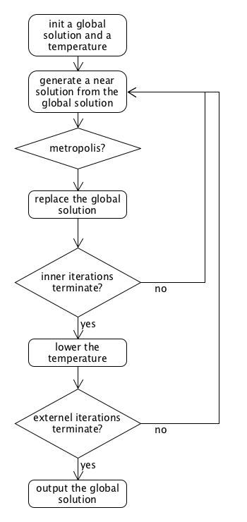
其中,内外层循环终止条件一般设定为经过一定数目的迭代次数后终止。
参数设定
- 初始温度
T=100 - 内层循环数为
1000 - 外层循环数为
1000 - 温度下降方式为
T *= 0.99
初始解的生成
初始全局解应当随机生成,即每个设施按均匀分布决定开或者不开。
邻域搜索
领域搜索即根据当前解生成下一个解,实验过程中发现模拟退火算法里使用多种邻域搜索方式共同作用比单种邻域搜索方式效果要好很多,实验中使用到的备选邻域操作有,
- 随机开启/关闭某个设施。
- 随机开启/关闭一段连续的设施。
- 将某一段连续的设施的开关状态倒置。
当需要生成新状态时,从上述三种方法中随机选择一种。
Metropolis 准则
Metropolis准则是模拟退火算法的核心所在,当这个准则满足时,接受生成的解并替换掉全局解。具体而言,Metropolis准则为
$$
\min\{1, e^{-\frac{C’-C}{T}}\} < R
$$
其中,$C’$为生成的解的费用,$C$为全局解的费用,$T$为温度,$R$为$[0,1]$之间的随机数。
可见,当遇到好解时,$e^{-\frac{C’-C}{T}} > 1$,必定会接收,但当遇到差解时,当温度高时,$e^{-\frac{C’-C}{T}}$比温度低时更加接近1,有概率接收此差解,且随着温度降低,接收差解的概率也降低,最终收敛到一个最优解。
复杂度分析
模拟退火算法的代码过程如下,
1 | func (s *Solver) solveBySA() *Solution { |
其中在内层循环,复制解的复杂度为$O(MN)$,随机邻域操作的平均复杂度为$O(N)$,其余均为常数时间,因此整体算法的时间复杂度为$O(EIMN)$,其中$E$为外层循环数,$I$为内层循环数。
由于整个过程只需保持一个解,空间复杂度为$O(MN)$。
实验结果
在71个问题的问题集上的实验结果如下,
| Result | Time(s) | |
|---|---|---|
| p1 | 8899.287 | 49.67533 |
| p2 | 7943.402 | 46.02201 |
| p3 | 9549.287 | 43.71652 |
| p4 | 10947.538 | 41.95468 |
| p5 | 8928.489 | 49.61210 |
| p6 | 7729.489 | 49.43371 |
| p7 | 9529.489 | 49.90450 |
| p8 | 11259.650 | 49.82498 |
| p9 | 8460.030 | 38.91396 |
| p10 | 7617.000 | 41.85766 |
| p11 | 9103.286 | 39.19025 |
| p12 | 10363.911 | 39.63912 |
| p13 | 8245.910 | 62.59881 |
| p14 | 7125.641 | 63.83618 |
| p15 | 8856.372 | 56.31368 |
| p16 | 10456.372 | 55.16921 |
| p17 | 8195.925 | 62.16191 |
| p18 | 7129.274 | 74.85285 |
| p19 | 8803.787 | 59.92987 |
| p20 | 10403.787 | 59.71305 |
| p21 | 8139.000 | 56.84904 |
| p22 | 7124.000 | 59.69487 |
| p23 | 8780.306 | 54.46691 |
| p24 | 10298.306 | 50.47274 |
| p25 | 12233.713 | 546.33127 |
| p26 | 11152.713 | 540.89889 |
| p27 | 13117.713 | 548.15456 |
| p28 | 15183.478 | 608.56645 |
| p29 | 13831.838 | 3797.52276 |
| p30 | 12366.202 | 666.75613 |
| p31 | 14535.702 | 642.78949 |
| p32 | 17277.047 | 629.18618 |
| p33 | 12174.419 | 531.56347 |
| p34 | 11212.667 | 585.61782 |
| p35 | 13843.667 | 565.90143 |
| p36 | 14570.419 | 500.77183 |
| p37 | 11424.636 | 427.68900 |
| p38 | 10594.000 | 512.98266 |
| p39 | 11976.636 | 429.34593 |
| p40 | 13176.636 | 428.54124 |
| p41 | 6755.391 | 100.04381 |
| p42 | 5680.069 | 93.40380 |
| p43 | 5401.000 | 80.17776 |
| p44 | 7162.573 | 113.07130 |
| p45 | 6244.500 | 104.98954 |
| p46 | 5994.292 | 95.73207 |
| p47 | 6424.425 | 127.02732 |
| p48 | 5594.600 | 125.31068 |
| p49 | 5304.300 | 98.86595 |
| p50 | 9258.967 | 139.52326 |
| p51 | 7748.878 | 198.40947 |
| p52 | 9862.039 | 167.22943 |
| p53 | 8969.800 | 165.41922 |
| p54 | 9331.120 | 136.80022 |
| p55 | 7789.517 | 157.08357 |
| p56 | 21422.086 | 1343.04327 |
| p57 | 26388.956 | 1220.42790 |
| p58 | 37722.381 | 1176.16916 |
| p59 | 27645.265 | 1169.97743 |
| p60 | 20923.000 | 1212.31783 |
| p61 | 25621.657 | 1052.55700 |
| p62 | 33197.623 | 957.01278 |
| p63 | 25287.956 | 975.96980 |
| p64 | 20834.000 | 1602.66377 |
| p65 | 25093.000 | 868.34070 |
| p66 | 32522.450 | 762.51041 |
| p67 | 24932.180 | 900.71575 |
| p68 | 20884.000 | 1051.84617 |
| p69 | 25202.000 | 937.94478 |
| p70 | 32858.727 | 845.59141 |
| p71 | 25924.628 | 923.64509 |
综合对比
三种算法在71个问题上的实验结果如下,您可以点击此链接下载所有解的详细结果,包括解的最终费用,开启的设施以及顾客的赋值情况。
| Result(greedy) | Time(s) | Result(brute-force) | Time(s) | Result(sa) | Time(s) | |
|---|---|---|---|---|---|---|
| p1 | 12989.953 | 0.00004 | 8899.287 | 0.01975 | 8899.287 | 49.67533 |
| p2 | 9288.850 | 0.00007 | 7943.402 | 0.01708 | 7943.402 | 46.02201 |
| p3 | 10488.850 | 0.00008 | 9543.402 | 0.01890 | 9549.287 | 43.71652 |
| p4 | 11688.850 | 0.00036 | 10947.538 | 0.01488 | 10947.538 | 41.95468 |
| p5 | 10902.060 | 0.00008 | 8928.489 | 0.00602 | 8928.489 | 49.61210 |
| p6 | 9832.666 | 0.00007 | 7729.489 | 0.00627 | 7729.489 | 49.43371 |
| p7 | 11432.666 | 0.00006 | 9529.489 | 0.00606 | 9529.489 | 49.90450 |
| p8 | 13032.666 | 0.00016 | 11259.081 | 0.00579 | 11259.650 | 49.82498 |
| p9 | 10980.250 | 0.00010 | 8460.030 | 0.03576 | 8460.030 | 38.91396 |
| p10 | 10458.043 | 0.00009 | 7617.000 | 0.03523 | 7617.000 | 41.85766 |
| p11 | 11458.043 | 0.00006 | 9103.286 | 0.03549 | 9103.286 | 39.19025 |
| p12 | 12458.043 | 0.00004 | 10363.911 | 0.03088 | 10363.911 | 39.63912 |
| p13 | 11015.048 | 0.00028 | 8245.910 | 63.38475 | 8245.910 | 62.59881 |
| p14 | 8514.791 | 0.00006 | 7125.641 | 63.63613 | 7125.641 | 63.83618 |
| p15 | 10114.791 | 0.00012 | 8856.372 | 62.66329 | 8856.372 | 56.31368 |
| p16 | 11714.791 | 0.00009 | 10456.372 | 61.17692 | 10456.372 | 55.16921 |
| p17 | 10295.318 | 0.00006 | 8195.925 | 60.36199 | 8195.925 | 62.16191 |
| p18 | 8543.171 | 0.00007 | 7100.582 | 69.37253 | 7129.274 | 74.85285 |
| p19 | 10143.171 | 0.00013 | 8803.787 | 66.69740 | 8803.787 | 59.92987 |
| p20 | 11743.171 | 0.00009 | 10403.787 | 60.53454 | 10403.787 | 59.71305 |
| p21 | 12235.528 | 0.00022 | 8054.758 | 64.53812 | 8139.000 | 56.84904 |
| p22 | 11363.414 | 0.00009 | 7092.000 | 64.51618 | 7124.000 | 59.69487 |
| p23 | 12563.414 | 0.00005 | 8740.758 | 64.48915 | 8780.306 | 54.46691 |
| p24 | 13763.414 | 0.00008 | 10267.971 | 64.60072 | 10298.306 | 50.47274 |
| p25 | 78338.667 | 0.00039 | - | $\infty$ | 12233.713 | 546.33127 |
| p26 | 63710.947 | 0.00032 | - | $\infty$ | 11152.713 | 540.89889 |
| p27 | 65310.947 | 0.00032 | - | $\infty$ | 13117.713 | 548.15456 |
| p28 | 66910.947 | 0.00034 | - | $\infty$ | 15183.478 | 608.56645 |
| p29 | 65258.221 | 0.00040 | - | $\infty$ | 13831.838 | 3797.52276 |
| p30 | 54927.860 | 0.00038 | - | $\infty$ | 12366.202 | 666.75613 |
| p31 | 56927.860 | 0.00043 | - | $\infty$ | 14535.702 | 642.78949 |
| p32 | 58927.860 | 0.00145 | - | $\infty$ | 17277.047 | 629.18618 |
| p33 | 77701.857 | 0.00035 | - | $\infty$ | 12174.419 | 531.56347 |
| p34 | 53887.154 | 0.00033 | - | $\infty$ | 11212.667 | 585.61782 |
| p35 | 55487.154 | 0.00035 | - | $\infty$ | 13843.667 | 565.90143 |
| p36 | 57087.154 | 0.00065 | - | $\infty$ | 14570.419 | 500.77183 |
| p37 | 101999.196 | 0.00024 | - | $\infty$ | 11424.636 | 427.68900 |
| p38 | 73636.480 | 0.00020 | - | $\infty$ | 10594.000 | 512.98266 |
| p39 | 74636.480 | 0.00022 | - | $\infty$ | 11976.636 | 429.34593 |
| p40 | 75636.480 | 0.00020 | - | $\infty$ | 13176.636 | 428.54124 |
| p41 | 7276.556 | 0.00021 | - | $\infty$ | 6755.391 | 100.04381 |
| p42 | 8068.351 | 0.00010 | - | $\infty$ | 5680.069 | 93.40380 |
| p43 | 6383.929 | 0.00009 | - | $\infty$ | 5401.000 | 80.17776 |
| p44 | 7995.223 | 0.00021 | - | $\infty$ | 7162.573 | 113.07130 |
| p45 | 8089.250 | 0.00013 | - | $\infty$ | 6244.500 | 104.98954 |
| p46 | 6915.251 | 0.00009 | - | $\infty$ | 5994.292 | 95.73207 |
| p47 | 7705.325 | 0.00015 | - | $\infty$ | 6424.425 | 127.02732 |
| p48 | 7874.275 | 0.00019 | - | $\infty$ | 5594.600 | 125.31068 |
| p49 | 6960.522 | 0.00009 | - | $\infty$ | 5304.300 | 98.86595 |
| p50 | 12441.358 | 0.00025 | - | $\infty$ | 9258.967 | 139.52326 |
| p51 | 9382.546 | 0.00034 | - | $\infty$ | 7748.878 | 198.40947 |
| p52 | 13378.456 | 0.00016 | - | $\infty$ | 9862.039 | 167.22943 |
| p53 | 12650.089 | 0.00019 | - | $\infty$ | 8969.800 | 165.41922 |
| p54 | 10536.867 | 0.00016 | - | $\infty$ | 9331.120 | 136.80022 |
| p55 | 12258.408 | 0.00019 | - | $\infty$ | 7789.517 | 157.08357 |
| p56 | 32522.303 | 0.00113 | - | $\infty$ | 21422.086 | 1343.04327 |
| p57 | 37322.303 | 0.00119 | - | $\infty$ | 26388.956 | 1220.42790 |
| p58 | 48522.303 | 0.00209 | - | $\infty$ | 37722.381 | 1176.16916 |
| p59 | 30606.927 | 0.00110 | - | $\infty$ | 27645.265 | 1169.97743 |
| p60 | 37243.427 | 0.00082 | - | $\infty$ | 20923.000 | 1212.31783 |
| p61 | 40543.427 | 0.00142 | - | $\infty$ | 25621.657 | 1052.55700 |
| p62 | 48243.427 | 0.00082 | - | $\infty$ | 33197.623 | 957.01278 |
| p63 | 31843.780 | 0.00091 | - | $\infty$ | 25287.956 | 975.96980 |
| p64 | 34081.806 | 0.00061 | - | $\infty$ | 20834.000 | 1602.66377 |
| p65 | 36481.806 | 0.00061 | - | $\infty$ | 25093.000 | 868.34070 |
| p66 | 42081.806 | 0.00063 | - | $\infty$ | 32522.450 | 762.51041 |
| p67 | 32210.447 | 0.00096 | - | $\infty$ | 24932.180 | 900.71575 |
| p68 | 38955.963 | 0.00073 | - | $\infty$ | 20884.000 | 1051.84617 |
| p69 | 41955.963 | 0.00071 | - | $\infty$ | 25202.000 | 937.94478 |
| p70 | 48955.963 | 0.00128 | - | $\infty$ | 32858.727 | 845.59141 |
| p71 | 31843.976 | 0.00096 | - | $\infty$ | 25924.628 | 923.64509 |
可以发现,模拟退火的算法要远好于贪心算法,并且与有结果的暴力求解的结果十分相近。