The simplest are also the most important.
Arrays and Linked Lists
In almost every programming language, arrays are built-in data structures. An array arranges continuous space for objects, and is good at random access. However, arrays perform bad when meet insertions and deletions, and cost a lot to change their sizes.
With a linked list, insertions and deletions are very fast to perform, but one cannot access objects randomly in a linked list with $O(1)$ time complexity.
Many complex data structures are implemented based on these two simple data structures.
Stacks
In a stack data structure, all insertions and deletions of entries are made at one end, called the top of the stack. When we add an item to a stack, we say that we push it onto the stack, and when we remove an item, we say that we pop it from the stack. Note that the last item pushed onto a stack is always the first that will be popped from the stack. This property is called last in, first out, or LIFO for short.
Stacks are simple enough to be understood by only a few sentences. The most important feature of a stack is the LIFO property, which is very useful when a task about reversal need to be performed.
Example: Reverse a List
When a series of objects need to be loaded and written out in reverse order, it's suitable to use a stack to accomplish the task. Consider a series of input as follow,
1 | 10 // The number of objects. |
A list in reverse order should be output like,
1 | 10,9,8,7,6,5,4,3,2,1 |
At this time, a perfect solution is using a stack. After pushing all the numbers into the stack, the reverse order of the list is automatically produced by popping them out.
Queues
For computer applications, we similarly define a queue to be a list in which all additions to the list are mode at one end, and all deletions from the list are made at the other end. Queues are also called first-in, first-out lists, or FIFO for short.
As a good brother of stacks, queues are also easy to understand. It's FIFO property is extremely suitable to perform tasks with particular orders, especially when some tasks need to wait for some other tasks.
Heaps
In a max heap, for any given node $C$, if $P$ is a parent node of $C$, then the key (the value) of $P$ is greater than or equal to the key of $C$. In a min heap, the key of $P$ is less than or equal to the key of $C$.
Heaps are often implemented by a binary tree, and a few important operations are listed below.
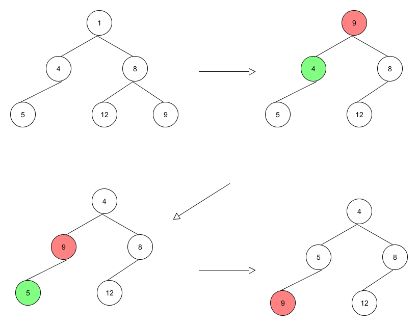
Insertion
To insert a new node to a heap, the general idea is to do swapping after the node is inserted to the "end".
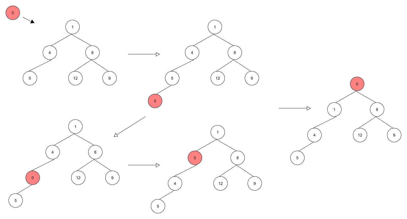
Deletion
Only the root can be deleted. We move the node in the "end" to the root and heapify.
Binary Trees
Binary trees are very powerful tools to solve difficult problems, but it is also difficult to determine when to use binary trees and what kinds of trees to use. Here some typical binary trees are introduced, but at first, let's remember the precise definition of a binary tree.
A binary tree is either empty, or it consists of a node called the root together with two binary trees called the left subtree and the right subtree of the root.
Binary Search Trees (BST)
A binary search tree is a binary tree that is either empty or in which every node has a key and satisfies the following conditions:
- The key of the root (if it exists) is greater than the key in any node in the left subtree of the root.
- The key of the root (if it exists) is less than the key in any node in the right substree of the root.
- The left and right subtrees of the root are again binary search trees.
We focus on the search, insertion and deletion of elements on a binary search tree.
Search is quite simple. Since the tree has the unequality property and is recursively defined, we can just use a simple recursive or iterative function to accomplish the task. Note that searching a key in the tree has a time complexity $O(log n)$.
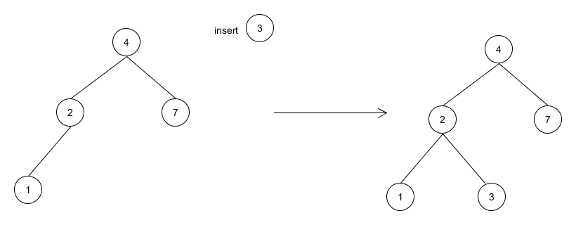
Insertion requires that after adding to new node to the tree, the tree is still a BST. However, since the tree is not required to be balanced, the process of insertion is quite like the process of search. We search in the tree as if the node has already been inserted, and when we reach a leaf node, we insert the node under that leaf node.
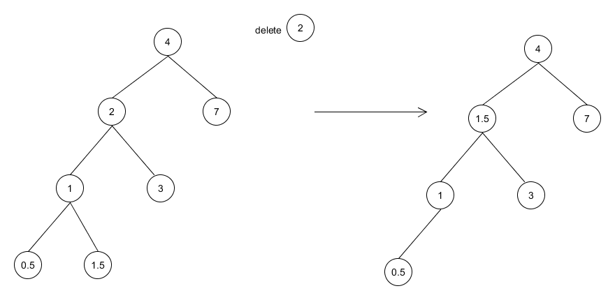
Deletion meets difficulties when a node with both left and right subtrees exist. At this time, we find the most farthest and most rightest child of the left subtree and replace it with the node. Since the child node is the greatest one of the left subtree and it is still less than any node on the right subtree, the replacement is safe. Note that this node may not be a leaf node but a node with only a left subtree, so a recursive deletion may occur.
AVL Trees
BSTs are no more than a good start point, because we cannot control the height of the tree when insertions or deletions occur frequently. AVL trees are mean to solve this problem, which can let a BST always be balanced.
An AVL tree is a binary search tree in which the heights of the left and right substrees of the root differ by at most 1 and in which the left and right subtrees are again AVL trees.
With each node of an AVL tree is associated a balance factor that is left-higher, equal-height, or right-higher according, respectively, as the left subtree has height greater than, equal to, or less than that of the right subtree.
The most important feature of an AVL tree is that it will perform some special operations, called rotations, in order to keep balance of the tree when insertions or deletions attempt to break the balance.
Let us first redefine the concept balance factor. Let $H_L(x)$ be the height of the left subtree of the node $x$, and $H_R(x)$ be the height of the right subtree. We say that the balance factor of node $x$
$$
bf(x) = H_L(x) - H_R(x)
$$
Therefore, any node $x$ of an AVL tree satisfies $|bf(x)| \le 1$.
When we meet a node $x$ that has a balance factor $|bf(x)| > 1$, generally there are four rotations like showing in the following table.
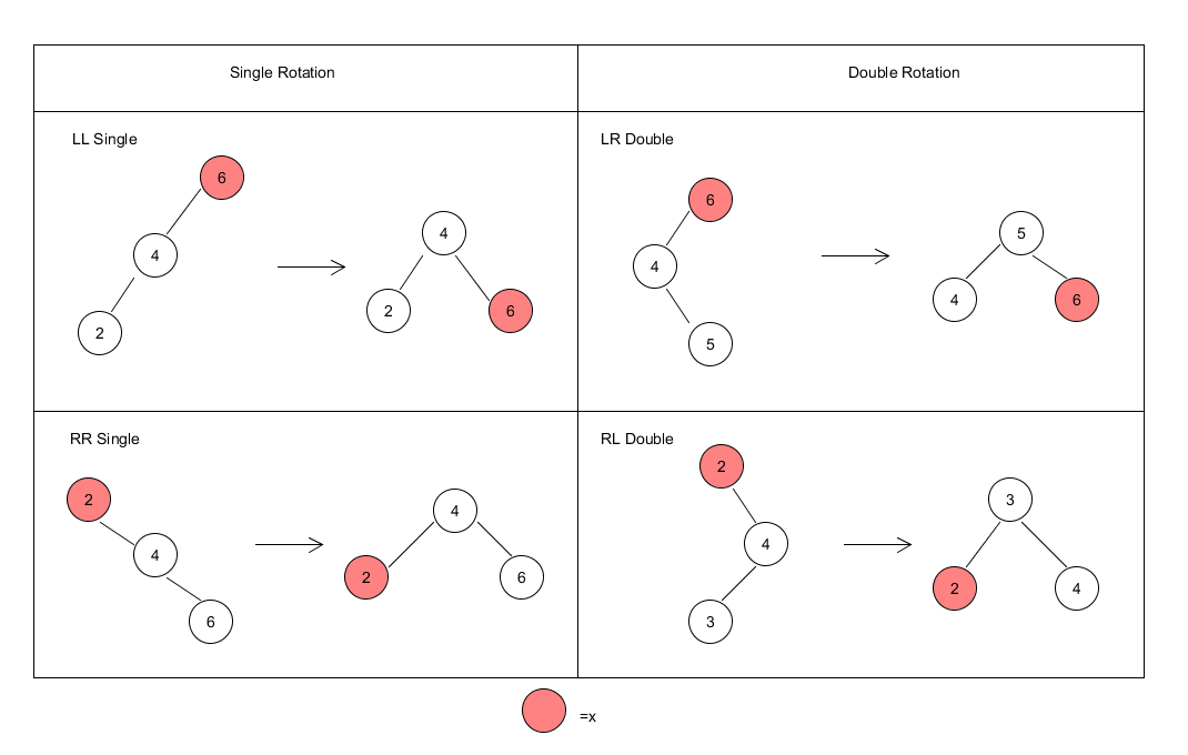
Insertion of a new node to an AVL tree has a new step after the node is inserted like a BST. First we insert the node as we insert the node to a BST, and then, we need to check the balance factor from the inserted node backward one by one. When we meet a node $x$ that has a balance factor $|bf(x)| > 1$, we stop immediately and perform a rotation to that node.
Deletion of a node in an AVL tree requires checking backward from the deleted node to the root node. If an unbalanced node is found, perform a rotation to that node.
Recursion
Recursion is the name for the case when a function invokes itself or invokes a sequence of other functions, one of which eventually invokes the first function again.
Recursion is a good way to fast accomplish a specific group of tasks like factorials. However, any recursive program can be rewritten to a iterative program with higher performance. Therefore, in modern software development, it is not a good idea to use recursion directly, but it is still worthwhile to learn because it provides a good method for us to find out answers of some complicated questions.
There are two main situations under which we may let recursion in. The first one is that we can write a formula which specify the relationship between the current state and one or a few previous states. Besides, an initial state is specified. For example, the factorials can be written like
$$
n! = \begin{cases}
1 &n = 0 \\
n(n - 1)! & n > 0
\end{cases}
$$
$n = 0$ is the initial state and when $n > 0$, the result is computed by $(n - 1)!$, a same problem but with a smaller scale.
Example: The Towers of Hanoi
If someone would like to teach recursion, he or she must introduce this typical problem – The Towers of Hanoi. This is a question that almost every one knows but, not all people can write down the solution immediately.
It is not so obvious that this problem is under the first situation, but we still can write down a formula here. Let m(n, s, d, t) represents "the steps move n disks from tower s to tower d using t as a temporary tower." Therefore, the formula can be written as
$$
m(n, s, d, t) = \begin{cases}
\text{do nothing} & n = 0 \\
m(n - 1, s, t, d) + m(1, s, d, t) + m(n - 1, t, d, s) & n > 0
\end{cases}
$$
The following is a simple C++ recursive program to accomplish the task.
1 | void move(int n, int s, int d, int t) { |
One more thing to say is that this program is terrible because every call produces two calls. Thus, with $n$ plates, the total number of calls is
$$
1 + 2 + 4 + \cdots + 2^{n - 1} = 2^n - 1
$$
Therefore, this is a program with $O(2^n)$ time complexity.
The second situation is that we need to do backtracking during the execution. In other words, we need to undo some operations that have already been done before. At this time, the structure of a recursive program is very useful. The next example is the typical Eight-Queens Puzzle, which will illustrate how the backtracking works.
Example: The Eight-Queens Puzzle
Computers are good at enumerating. When they meet the Eight-Queens Puzzle, they simply try all possible positions row by row. Obviously, it is easy to reach a dead end and a backtracking need to be performed, so we use a recursive structure to accomplish the task.
The following is a simple C++ recursive program to solve the puzzle.
1 | // The board is a 8x8 array with 0 representing empty and 1 representing |
Can you find all solutions of the Eight-Queens Puzzle?
Searching
Every one knows the general idea of binary search. The problem is that when to use it to reduce the time complexity of a program. Here I would like to introduce a "standard" implementation of binary search. Note that even the general idea of binary search is the same, the actual times of comparison may still vary from implementations to implementations.
Here is the code of searching in a sorted vector of integers.
1 | int binarySearch(vector<int> &nums, int target) { |
Sorting
Sorting is a very facinating topic in the field of algorithms. It can be simple, like perform a selection sort on a list of integers, and suitable for newcommers to learn. It is also worth thinking because the mergesort and the quicksort are two of the most typical algorithms applying the divide-and-conquer method, which are widely used in plenty of tasks. It is extremely useful because it can reduce the time complexity of searching. It also provides judgements of performances of other algorithms. In conclusion, it is worthwhile to learn sorting as many times as you can and to remember it in your heart.
I am not going to introduce sorting algorithms with $O(n^2)$ time complexity like selection sort or bubble sort. I will main focus on quicksort and mergesort here.
Mergesort
In the first method, we simply chop the list into two sublists of sizes as nearly equal as possible and then sort them separately. Afterward, we carefully merge the two sorted sublists into a single sorted list.
The main procedure of mergesort is to divide the list into two sublists and perform mergesort on each sublist, repectively. Then the sublists will be merged to a sorted list. This process is recursive. When a sublist only contains one element, this sublist is automatically sorted and the combination begins immediately.
The following is a common recursive C++ implementation to sort a vector of integers.
1 | void recursiveMergeSort(vector<int> &nums, int left, int right) { |
References
Robert L. K. and Alexander J. R., Data Structures and Program Design in C++.